OS Concepts

Operating System

An Operating System (OS) is a collection of software that manages computer hardware and provides services for programs. Specifically, it hides hardware complexity, manages computational resources, and provides isolation and protection. Most importantly, it directly has privilege access to the underlying hardware. Major components of an OS are file system, scheduler, and device driver. You probably have used both Desktop (Windows, Mac, Linux) and Embedded (Android, iOS) operating systems before.

There are 3 key elements of an operating system, which are: (1) Abstractions (process, thread, file, socket, memory), (2) Mechanisms (create, schedule, open, write, allocate), and (3) Policies (LRU, EDF)

There are 2 operating system design principles, which are: (1) Separation of mechanism and policy by implementing flexible mechanisms to support policies, and (2) Optimize for common case: Where will the OS be used? What will the user want to execute on that machine? What are the workload requirements?

The 3 types of Operating Systems commonly used nowadays are: (1) Monolithic OS, where the entire OS is working in kernel space and is alone in supervisor mode; (2) Modular OS, in which some part of the system core will be located in independent files called modules that can be added to the system at run time; and (3) Micro OS, where the kernel is broken down into separate processes, known as servers. Some of the servers run in kernel space and some run in user-space.

Boot Process

When a system is first booted, or is reset, the processor executes code at a well-known location. In a personal computer (PC), this location is in the basic input/output system (BIOS), which is stored in flash memory on the motherboard. The central processing unit (CPU) in an embedded system invokes the reset vector to start a program at a known address in flash/ROM. In either case, the result is the same. Because PCs offer so much flexibility, the BIOS must determine which devices are candidates for boot.

When a boot device is found, the first-stage boot loader is loaded into RAM and executed. This boot loader is less than 512 bytes in length (a single sector), and its job is to load the second-stage boot loader.

When the second-stage boot loader is in RAM and executing, a splash screen is commonly displayed, and Linux and an optional initial RAM disk (temporary root file system) are loaded into memory. When the images are loaded, the second-stage boot loader passes control to the kernel image and the kernel is decompressed and initialized. At this stage, the second-stage boot loader checks the system hardware, enumerates the attached hardware devices, mounts the root device, and then loads the necessary kernel modules. When complete, the first user-space program (init) starts, and high-level system initialization is performed.

System startup

The system startup stage depends on the hardware that Linux is being booted on. On an embedded platform, a bootstrap environment is used when the system is powered on, or reset. Examples include U-Boot, RedBoot, and MicroMonitor from Lucent. Embedded platforms are commonly shipped with a boot monitor. These programs reside in special region of flash memory on the target hardware and provide the means to download a Linux kernel image into flash memory and subsequently execute it. In addition to having the ability to store and boot a Linux image, these boot monitors perform some level of system test and hardware initialization. In an embedded target, these boot monitors commonly cover both the first- and second-stage boot loaders.

In a PC, booting Linux begins in the BIOS at address 0xFFFF0. The first step of the BIOS is the power-on self test (POST). The job of the POST is to perform a check of the hardware. The second step of the BIOS is local device enumeration and initialization.

Given the different uses of BIOS functions, the BIOS is made up of two parts: the POST code and runtime services. After the POST is complete, it is flushed from memory, but the BIOS runtime services remain and are available to the target operating system.

To boot an operating system, the BIOS runtime searches for devices that are both active and bootable in the order of preference defined by the complementary metal oxide semiconductor (CMOS) settings. A boot device can be a floppy disk, a CD-ROM, a partition on a hard disk, a device on the network, or even a USB flash memory stick.

Commonly, Linux is booted from a hard disk, where the Master Boot Record (MBR) contains the primary boot loader. The MBR is a 512-byte sector, located in the first sector on the disk (sector 1 of cylinder 0, head 0). After the MBR is loaded into RAM, the BIOS yields control to it.

Stage 1 boot loader

The primary boot loader that resides in the MBR is a 512-byte image containing both program code and a small partition table (see Figure 2). The first 446 bytes are the primary boot loader, which contains both executable code and error message text. The next sixty-four bytes are the partition table, which contains a record for each of four partitions (sixteen bytes each). The MBR ends with two bytes that are defined as the magic number (0xAA55). The magic number serves as a validation check of the MB

The job of the primary boot loader is to find and load the secondary boot loader (stage 2). It does this by looking through the partition table for an active partition. When it finds an active partition, it scans the remaining partitions in the table to ensure that they’re all inactive. When this is verified, the active partition’s boot record is read from the device into RAM and executed.

Stage 2 boot loader

The secondary, or second-stage, boot loader could be more aptly called the kernel loader. The task at this stage is to load the Linux kernel and optional initial RAM disk

The first- and second-stage boot loaders combined are called Linux Loader (LILO) or GRand Unified Bootloader (GRUB) in the x86 PC environment. Because LILO has some disadvantages that were corrected in GRUB, let’s look into GRUB.

The great thing about GRUB is that it includes knowledge of Linux file systems. Instead of using raw sectors on the disk, as LILO does, GRUB can load a Linux kernel from an ext2 or ext3 file system. It does this by making the two-stage boot loader into a three-stage boot loader. Stage 1 (MBR) boots a stage 1.5 boot loader that understands the particular file system containing the Linux kernel image. Examples include reiserfs_stage1_5 (to load from a Reiser journaling file system) or e2fs_stage1_5 (to load from an ext2 or ext3 file system). When the stage 1.5 boot loader is loaded and running, the stage 2 boot loader can be loaded.

With stage 2 loaded, GRUB can, upon request, display a list of available kernels (defined in /etc/grub.conf, with soft links from /etc/grub/menu.lst and /etc/grub.conf). You can select a kernel and even amend it with additional kernel parameters. Optionally, you can use a command-line shell for greater manual control over the boot process.

With the second-stage boot loader in memory, the file system is consulted, and the default kernel image and initrd image are loaded into memory. With the images ready, the stage 2 boot loader invokes the kernel image.

Kernel

With the kernel image in memory and control given from the stage 2 boot loader, the kernel stage begins. The kernel image isn’t so much an executable kernel, but a compressed kernel image. Typically this is a zImage (compressed image, less than 512KB) or a bzImage (big compressed image, greater than 512KB), that has been previously compressed with zlib. At the head of this kernel image is a routine that does some minimal amount of hardware setup and then decompresses the kernel contained within the kernel image and places it into high memory. If an initial RAM disk image is present, this routine moves it into memory and notes it for later use. The routine then calls the kernel and the kernel boot begins.

Init

After the kernel is booted and initialized, the kernel starts the first user-space application. This is the first program invoked that is compiled with the standard C library. Prior to this point in the process, no standard C applications have been executed.

In a desktop Linux system, the first application started is commonly /sbin/init. But it need not be. Rarely do embedded systems require the extensive initialization provided by init (as configured through /etc/inittab). In many cases, you can invoke a simple shell script that starts the necessary embedded applications.

Process and Process Management

A process is an instance of a program being executed (a running program). They allow for a single processor to run multiple programs "simulatneously". Each process runs on a virtual CPU, and the real CPU can use this to run any single process. Effectively, the single CPU has been divided into multiple virtual CPUs.

Why have Processes?

They:

• provide an illusion of concurrency.
• provide isolation between programs (each process has its own address space).
• simplify programming (programs don't have to worry about other programs).
• allow for better utilisation of resources (different processes require different resources at certain times).

Time-Slicing for Concurrency

An OS can switch the current running process every few milliseconds such that every process can have CPU time. This is done using a CPU scheduler, and it can be used to provide pseudo concurrency.

Types of Concurrency

Pseudo Concurrency: a single processor switches between processes by interleaving their runtimes. Overtime this can give the illusion of concurrent execution.

Real Concurrency: multiple processors or CPU cores are used to run multiple processes in parallel.

Fairness

Fairness is the concept that the CPU scheduler switches fairly between processes. This means that every process should have equal CPU time, or more generally they should have appropriate CPU times determined by each processes priority and workload.

Context Switches

A context switch is when a processor switches from executing one process to another.

An OS may switch either periodically or in reponse to certain events / interrupts (such as I/O completion). Context switches are not pre-determined because the events causing them are non-deterministic.

Since processes will need to be restarted safely when being switched to, all relevant information (e.g. register values) must be stored when they are switched away from. This is done by storing the data in a process descriptor or a process control block (PCB), which is kept inside a process table.

Context switches are expensive. The process state needs to be saved / restored and CPU caches (including translation lookaside buffer (TLB)) will be lost. It is important for an OS to avoid unnecessary context switches.

Process Control Block (PCB)

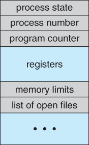
Each process has it's own virtual machine: They have their own virtual CPU, address space (stack, heap, text, data, etc), open file descriptors, etc. Enough data must be stored such that all of this remains preserved after a context switch.

The information that gets stored on a context switch is:

• Registers: program counter (PC), page table register, stack pointer, etc.
• Process management info: process ID (PID), parent process, process group, priority, CPU used, etc.
• File management info: root directory, working directory, open file descriptors, etc.

Stack

Stack memory is responsible for housing control information, local variables, and function arguments, including return addresses.Stack memory is responsible for housing control information, local variables, and function arguments, including return addresses. The stack is a "FILO" (first in, last out) data structure, that is managed and optimized by the CPU quite closely. Every time a function declares a new variable, it is "pushed" onto the stack. Then every time a function exits, all of the variables pushed onto the stack by that function, are freed (that is to say, they are deleted). Once a stack variable is freed, that region of memory becomes available for other stack variables.

The advantage of using the stack to store variables, is that memory is managed for you. You don't have to allocate memory by hand, or free it once you don't need it any more. What's more, because the CPU organizes stack memory so efficiently, reading from and writing to stack variables is very fast.

A key to understanding the stack is the notion that when a function exits, all of its variables are popped off of the stack (and hence lost forever). Thus stack variables are local in nature. This is related to a concept we saw earlier known as variable scope, or local vs global variables. A common bug in C programming is attempting to access a variable that was created on the stack inside some function, from a place in your program outside of that function (i.e. after that function has exited).

Another feature of the stack to keep in mind, is that there is a limit (varies with OS) on the size of variables that can be store on the stack. This is not the case for variables allocated on the heap.

Heap

The heap is a region of your computer's memory that is not managed automatically for you, and is not as tightly managed by the CPU. Heap memory, also known as dynamic memory, is the wild child of memory allocation. The programmer has to manage it manually. Heap memory allows us to allocate and free up memory at any time during our program's execution. It's great for storing large data structures or objects whose sizes aren't known in advance. To allocate memory on the heap, you must use malloc() or calloc(), which are built-in C functions. Once you have allocated memory on the heap, you are responsible for using free() to deallocate that memory once you don't need it any more. If you fail to do this, your program will have what is known as a memory leak. That is, memory on the heap will still be set aside (and won't be available to other processes). As we will see in the debugging section, there is a tool called valgrind that can help you detect memory leaks.

Unlike the stack, the heap does not have size restrictions on variable size (apart from the obvious physical limitations of your computer). Heap memory is slightly slower to be read from and written to, because one has to use pointers to access memory on the heap. We will talk about pointers shortly.

Unlike the stack, variables created on the heap are accessible by any function, anywhere in your program. Heap variables are essentially global in scope.

Creating Processes

int fork(void)

fork creates a new child process by making an exact copy of the parent process image. The child process inherits its parent's resources and will begin to execute concurrently with it.

fork returns twice, once in the parent, and once in the child:

• Parent: return value is the process ID of the child.
• Child: return value is 0.
• Error: if fork is unable to create a child, -1 is returned to the parent. This can happen if there isn't enough memory to create the child process in.

An example of some code using fork:

#include <unistd.h>
#include <stdio.h>

int main() {
  if (fork() != 0) {
    printf("Parent process\n");
  } else {
    printf("Child process\n");
  }

  printf("Common code\n");
}

Executing Processes

int execve(
  const char *path,
  char *const argv[],
  char *const envp[]
)

execve executes a command. Instead of copying the parent process, a completely new process is made.

Its arguments are:

• path: the full pathname of the program to be executed.
• argv: the arguments passed to this program.
• envp: a list of environment variables.

execve has many useful wrappers (execl, execle, execvp, execv, etc). Read man execve for more.

Waiting for Process Termination

int waitpid(
  int pid,
  int* stat,
  int options
)

waitpid suspends execution of the calling process until the child process with the PID terminates normally or it receives a signal.

waitpid can be used to wait for multiple children:

• pid = -1: wait for any child.
• pid = 0 wait for any child in the same process group as caller.
• pid = -gid wait for any child with process group gid.

Its return value can be:

• the pid of the terminated child process.
• 0 if WNOHANG is set in options. This option "is used to indicate that the call should not block if there are no processes that wish to report status" (from man waitpid).
• -1 on error, and errno is set to indicate the error (see man errno).

Process Termination

void exit(int status)

exit terminates the calling process, returning the exit status to the parent process (i.e. through int *stat in waitpid).

void kill(int pid, int sid)

kill sends signal sig to process with PID pid.

An example of exit:

#include <unistd.h>
#include <sys/wait.h>
#include <stdio.h>
#include <stdlib.h>

int main() {
  int pid = fork();

  if (pid != 0) {
    // parent process
    int *stat;
    waitpid(pid, stat, 0);
    printf("Child exit status is: %d\n", WEXITSTATUS(*stat));
  } else {
    // child process
    exit(4);
  }
}

$ gcc a.c && ./a.out
Child exit status is: 4

Process Hierarchies

UNIX allows for processes to form hierarchies (e.g. parent, child, child's child, etc).

Windows has no notion of process hierarchy. Instead when a process is created its parent is given a handle token to control it. This handle can be passed around to other processes.

Process States

• Zombie: has completed execution, still has an entry in the process table
• Orphan: parent has finished or terminated while this process is still running
• Daemon: runs as a background process, not under the direct control of an interactive user.

Zombie Process

On Unix and Unix-like computer operating systems, a zombie process or defunct process is a process that has completed execution (via the exit system call) but still has an entry in the process table: it is a process in the "Terminated state".

This occurs for child processes, where the entry is still needed to allow the parent process to read its child's exit status: once the exit status is read via the wait system call, the zombie's entry is removed from the process table and it is said to be "reaped". A child process always first becomes a zombie before being removed from the resource table.

In most cases, under normal system operation zombies are immediately waited on by their parent and then reaped by the system – processes that stay zombies for a long time are generally an error and cause a resource leak.

The term zombie process derives from the common definition of zombie — an undead person. In the term's metaphor, the child process has "died" but has not yet been "reaped". Also, unlike normal processes, the kill command has no effect on a zombie process.

Zombie processes should not be confused with orphan processes: an orphan process is a process that is still executing, but whose parent has died. These do not remain as zombie processes; instead, (like all orphaned processes) they are adopted by init (process ID 1), which waits on its children. The result is that a process that is both a zombie and an orphan will be reaped automatically.

Linux Signals

In Linux, every signal has a name that begins with characters SIG. For example :

• A SIGINT signal that is generated when a user presses ctrl+c. This is the way to terminate programs from terminal.
• A SIGALRM is generated when the timer set by alarm function goes off.
• A SIGABRT signal is generated when a process calls the abort function. etc

When the signal occurs, the process has to tell the kernel what to do with it. There can be three options through which a signal can be disposed:

• The signal can be ignored. By ignoring we mean that nothing will be done when signal occurs. Most of the signals can be ignored but signals generated by hardware exceptions like divide by zero, if ignored can have weird consequences. Also, a couple of signals like SIGKILL and SIGSTOP cannot be ignored.

• The signal can be caught. When this option is chosen, then the process registers a function with kernel. This function is called by kernel when that signal occurs. If the signal is non fatal for the process then in that function the process can handle the signal properly or otherwise it can chose to terminate gracefully. Let the default action apply. Every signal has a default action. This could be process terminate, ignore etc.

• As we already stated that two signals SIGKILL and SIGSTOP cannot be ignored. This is because these two signals provide a way for root user or the kernel to kill or stop any process in any situation .The default action of these signals is to terminate the process. Neither these signals can be caught nor can be ignored.

What Happens at Program Start-up?

It all depends on the process that calls exec. When the process is started the status of all the signals is either ignore or default. Its the later option that is more likely to happen unless the process that calls exec is ignoring the signals.

It is the property of exec functions to change the action on any signal to be the default action. In simpler terms, if parent has a signal catching function that gets called on signal occurrence then if that parent execs a new child process, then this function has no meaning in the new process and hence the disposition of the same signal is set to the default in the new process.

Also, Since we usually have processes running in background so the shell just sets the quit signal disposition as ignored since we do not want the background processes to get terminated by a user pressing a ctrl+c key because that defeats the purpose of making a process run in background.

Threads and Concurrency

A thread is a subset of the process. It is termed as a ‘lightweight process’, since it is similar to a real process but executes within the context of a process and shares the same resources allotted to the process by the kernel. Usually, a process has only one thread of control – one set of machine instructions executing at a time. A process may also be made up of multiple threads of execution that execute instructions concurrently. Multiple threads of control can exploit the true parallelism possible on multiprocessor systems. All the threads running within a process share the same address space, file descriptors, stack and other process related attributes. Since the threads of a process share the same memory, synchronizing the access to the shared data withing the process gains unprecedented importance.

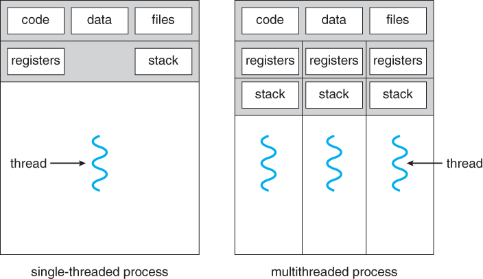
A break down of per process and per thread items is:

Per process items:

• Address space.
• Global variables.
• Open files.
• Child processes.
• Signals.

Per thread items:

• Program counter (PC).
• Registers.
• Stack.

Benefits of Multi-threading

• Parallelization: In multi-processor architecture, different threads can execute different instructions at a time, which result in parallelization which speeds up the execution of the process.

• Specialization: By specializing different threads to perform the different task, we can manage threads, for example, we can give higher priority to those threads which are executing the more important task. Also in multi-processor architecture specialization leads to the hotter cache which improves performance.

• Efficient: Multi-threaded programs are more efficient as compared to multi-process programs in terms of resource requirement as threads share address space while process does not, so multi-process programs will require separate memory space allocation. Also, Multi-threaded programs incur lower overhead as inter-thread communication is less expensive.

• Hide Latency: As context switching among the process is a costly operation, as all the threads of a process share the same virtual to physical address mapping and other resources, context switch among the thread is a cheap operation and require less time. When the number of thread is greater than the number of CPU and a thread is in idle state (spending the time to wait for the result of some interrupt) and its idle time is greater than two times the time required for switching the context to another thread, it will switch the switch context to another thread to hide idling time.

Problems / Concerns with Threads

• Threads have a shared address space. This means that they don't have any protection from reading / writing to each others stack like processes have. This can cause memory corruption issues and other concurrency bugs due to concurrent access to shared data (e.g. through global variables).

If one thread forks, is the entire process copied, or is the new process single-threaded?

A: It is system dependant. If the new process execs right away, there is no need to copy all the other threads. If it doesn't, then the entire process should be copied. Many versions of UNIX provide multiple versions of the fork call for this purpose.

Handling signals also becomes an issue. Which thread should handle the signal?

There are four major options:

1. Deliver the signal to the thread to which the signal applies.
2. Deliver the signal to every thread in the process.
3. Deliver the signal to certain threads in the process.
4. Assign a specific thread to receive all signals in a process.

Scheduling

Linux scheduling is based on the time sharing technique: several processes run in “time multiplexing” because the CPU time is divided into slices, one for each runnable process. If a currently running process is not terminated when its time slice or quantum expires, a process switch may take place. Time sharing relies on timer interrupts and is thus transparent to processes. No additional code needs to be inserted in the programs to ensure CPU time sharing.

The Linux scheduler is a priority based scheduler that schedules tasks based upon their static and dynamic priorities. When these priorities are combined they form a task's goodness . Each time the Linux scheduler runs, every task on the run queue is examined and its goodness value is computed. The task with the highest goodness is chosen to run next.

When there are cpu bound tasks running in the system, the Linux scheduler may not be called for intervals of up to .40 seconds. This means that the currently running task has the CPU to itself for periods of up to .40 seconds (how long depends upon the task's priority and whether it blocks or not). This is good for throughput because there are few computationally uneccessary context switches. However it can kill interactivity because Linux only reschedules when a task blocks or when the task's dynamic priority (counter) reaches zero. Thus under Linux's default priority based scheduling method, long scheduling latencies can occur.

Looking at the scheduling latency in finer detail, the Linux scheduler makes use of a timer that interrupts every 10 msec. This timer erodes the currently running task's dynamic priority (decrements its counter). A task's counter starts out at the same value its priority contains. Once its dynamic priority (counter) has eroded to 0 it is again reset to that of its static priority (priority). It is only after the counter reaches 0 that a call to schedule() is made. Thus a task with the default priority of 20 may run for .200 secs (200 msecs) before any other task in the system gets a chance to run. A task at priority 40 (the highest priority allowed) can run for .400 secs without any scheduling occurring as long as it doesn't block or yield.

Process scheduling is an essential part of a Multiprogramming operating systems. Such operating systems allow more than one process to be loaded into the executable memory at a time and the loaded process shares the CPU using time multiplexing.

Memory Management

• It should be noted that from the memory chips point of view, all memory accesses are equivalent. The memory hardware doesn't know what a particular part of memory is being used for, nor does it care. This is almost true of the OS as well, although not entirely.

• The CPU can only access its registers and main memory. It cannot, for example, make direct access to the hard drive, so any data stored there must first be transferred into the main memory chips before the CPU can work with it. ( Device drivers communicate with their hardware via interrupts and "memory" accesses, sending short instructions for example to transfer data from the hard drive to a specified location in main memory. The disk controller monitors the bus for such instructions, transfers the data, and then notifies the CPU that the data is there with another interrupt, but the CPU never gets direct access to the disk. )

• Memory accesses to registers are very fast, generally one clock tick, and a CPU may be able to execute more than one machine instruction per clock tick.

• Memory accesses to main memory are comparatively slow, and may take a number of clock ticks to complete. This would require intolerable waiting by the CPU if it were not for an intermediary fast memory cache built into most modern CPUs. The basic idea of the cache is to transfer chunks of memory at a time from the main memory to the cache, and then to access individual memory locations one at a time from the cache.

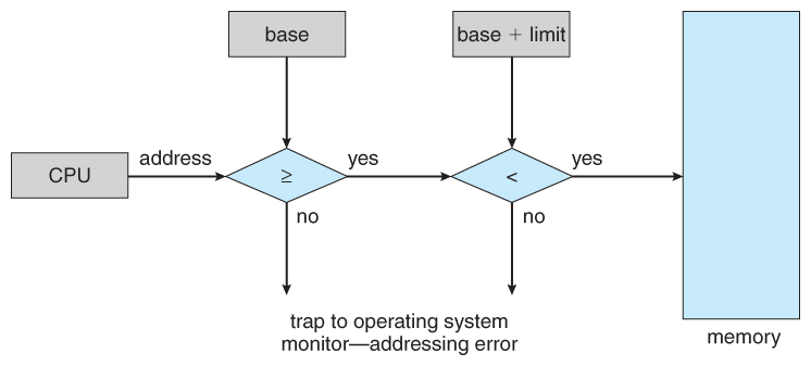
• User processes must be restricted so that they only access memory locations that "belong" to that particular process. This is usually implemented using a base register and a limit register for each process, as shown in Figures 8.1 and 8.2 below. Every memory access made by a user process is checked against these two registers, and if a memory access is attempted outside the valid range, then a fatal error is generated. The OS obviously has access to all existing memory locations, as this is necessary to swap users' code and data in and out of memory. It should also be obvious that changing the contents of the base and limit registers is a privileged activity, allowed only to the OS kernel.

Logical vs Physical Address Space

• The address generated by the CPU is a logical address, whereas the address actually seen by the memory hardware is a physical address.

• Addresses bound at compile time or load time have identical logical and physical addresses.

• Addresses created at execution time, however, have different logical and physical addresses.

  • In this case the logical address is also known as a virtual address, and the two terms are used interchangeably by our text.
  • The set of all logical addresses used by a program composes the logical address space, and the set of all corresponding physical addresses composes the physical address space.

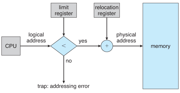
• The run time mapping of logical to physical addresses is handled by the memory-management unit, MMU.

  • The MMU can take on many forms. One of the simplest is a modification of the base-register scheme described earlier.
  • The base register is now termed a relocation register, whose value is added to every memory request at the hardware level.

Note that user programs never see physical addresses. User programs work entirely in logical address space, and any memory references or manipulations are done using purely logical addresses. Only when the address gets sent to the physical memory chips is the physical memory address generated.

Locality

Because memory devices vary considerably in their performance characteristics and storage capacities, modern systems integrate several forms of storage. Luckily, most programs exhibit common memory access patterns, known as locality, and designers build hardware that exploits good locality to automatically move data into an appropriate storage location. Specifically, a system improves performance by moving the subset of data that a program is actively using into storage that lives close to the CPU’s computation circuitry (for example, in a register or CPU cache). As necessary data moves up the hierarchy toward the CPU, unused data moves farther away to slower storage until the program needs it.

Systems primarily exploit two forms of locality:

• Temporal locality: Programs tend to access the same data repeatedly over time. That is, if a program has used a variable recently, it’s likely to use that variable again soon.

• Spatial locality: Programs tend to access data that is nearby other, previously accessed data. "Nearby" here refers to the data’s memory address. For example, if a program accesses data at addresses N and N+4, it’s likely to access N+8 soon.

In many cases, a programmer can help a system by intentionally writing code that exhibits good locality patterns. For example, consider the nested loops that access every element of an N×N matrix (this same example appeared in this chapter’s introduction):

float averageMat_v1(int **mat, int n) {
    int i, j, total = 0;

    for (i = 0; i < n; i++) {
        for (j = 0; j < n; j++) {
            // Note indexing: [i][j]
            total += mat[i][j];
        }
    }

    return (float) total / (n * n);
}

float averageMat_v2(int **mat, int n) {
    int i, j, total = 0;

    for (i = 0; i < n; i++) {
        for (j = 0; j < n; j++) {
            // Note indexing: [j][i]
            total += mat[j][i];
        }
    }

    return (float) total / (n * n);
}

In both versions, the loop variables (i and j) and the accumulator variable (total) exhibit good temporal locality because the loops repeatedly use them in every iteration. Thus, when executing this code, a system would store those variables in fast on-CPU storage locations to provide good performance.

However, due to the row-major order organization of a matrix in memory, the first version of the code (left) executes about five times faster than the second version (right). The disparity arises from the difference in spatial locality — the first version accesses the matrix’s values sequentially in memory (that is, in order of consecutive memory addresses). Thus, it benefits from a system that loads large blocks from memory into the cache because it pays the cost of going to memory only once for every block of values.

The second version accesses the matrix’s values by repeatedly jumping between rows across nonsequential memory addresses. It never reads from the same cache block in subsequent memory accesses, so it looks to the cache like the block isn’t needed. Thus, it pays the cost of going to memory for every matrix value it reads.

Contiguous Memory Allocation

One approach to memory management is to load each process into a contiguous space. The operating system is allocated space first, usually at either low or high memory locations, and then the remaining available memory is allocated to processes as needed.

The system shown below allows protection against user programs accessing areas that they should not, allows programs to be relocated to different memory starting addresses as needed, and allows the memory space devoted to the OS to grow or shrink dynamically as needs change.

Memory Allocation

One method of allocating contiguous memory is to divide all available memory into equal sized partitions, and to assign each process to their own partition. This restricts both the number of simultaneous processes and the maximum size of each process, and is no longer used.

An alternate approach is to keep a list of unused ( free ) memory blocks ( holes ), and to find a hole of a suitable size whenever a process needs to be loaded into memory. There are many different strategies for finding the "best" allocation of memory to processes, including the three most commonly discussed:

• First fit - Search the list of holes until one is found that is big enough to satisfy the request, and assign a portion of that hole to that process. Whatever fraction of the hole not needed by the request is left on the free list as a smaller hole. Subsequent requests may start looking either from the beginning of the list or from the point at which this search ended.
• Best fit - Allocate the smallest hole that is big enough to satisfy the request. This saves large holes for other process requests that may need them later, but the resulting unused portions of holes may be too small to be of any use, and will therefore be wasted. Keeping the free list sorted can speed up the process of finding the right hole.
• Worst fit - Allocate the largest hole available, thereby increasing the likelihood that the remaining portion will be usable for satisfying future requests.

Simulations show that either first or best fit are better than worst fit in terms of both time and storage utilization. First and best fits are about equal in terms of storage utilization, but first fit is faster.

Fragmentation

All the memory allocation strategies suffer from external fragmentation, though first and best fits experience the problems more so than worst fit. External fragmentation means that the available memory is broken up into lots of little pieces, none of which is big enough to satisfy the next memory requirement, although the sum total could.

The amount of memory lost to fragmentation may vary with algorithm, usage patterns, and some design decisions such as which end of a hole to allocate and which end to save on the free list.

Statistical analysis of first fit, for example, shows that for N blocks of allocated memory, another 0.5 N will be lost to fragmentation.

Internal fragmentation also occurs, with all memory allocation strategies. This is caused by the fact that memory is allocated in blocks of a fixed size, whereas the actual memory needed will rarely be that exact size. For a random distribution of memory requests, on the average 1/2 block will be wasted per memory request, because on the average the last allocated block will be only half full.

If the programs in memory are relocatable, ( using execution-time address binding ), then the external fragmentation problem can be reduced via compaction, i.e. moving all processes down to one end of physical memory. This only involves updating the relocation register for each process, as all internal work is done using logical addresses.

Another solution as we will see in is to allow processes to use non-contiguous blocks of physical memory, with a separate relocation register for each block.

Paging

Paging allows for the logical address space to be noncontiguous, so a process can allocate physical memory when it is needed / available.

Paging has two important concepts, frames and pages:

• Frames: a fixed-size block of physical memory.
• Pages: a block of logical (virtual) memory, the same size as a frame.

A typical page size is 4KB.

When a program of n pages is run:

1. n free frames are found.
2. the program is loaded into this memory.
3. a page table is setup to translate logical addresses to physical addresses.

Page Table

A page table is a translation mechanism from logical memory to physical memory.

    Virtual        Page         Physical
    Memory         Table         Memory
  *--------*       *---*       *--------*
  | Page 0 |     0 | 1 |     0 |        |
  *--------*       *---*       *--------*
  | Page 1 |     1 | 4 |     1 | Page 0 |
  *--------*       *---*       *--------*
  | Page 2 |     2 | 3 |     2 |        |
  *--------*       *---*       *--------*
  | Page 3 |     3 | 7 |     3 | Page 2 |
  *--------*    /  *---*       *--------*
               /     |       4 | Page 1 |
              /      |         *--------*
           Page      |       5 |        |
          Number     |         *--------*
                     *       6 |        |
                    /          *--------*
               Frame ------- 7 | Page 3 |
               Number          *--------*

Address Translation

When translating an address, the page table can be used to find the frame that the data exists in, but the offset inside the frame is also required. This offset is equal to the offset inside the page as they are equal size.

Logical addresses can be split into two sections:

• Page number p: used as the index to the page table. The page table only stores the base address of the page in physical memory.
• Page offset d: combined with the base address of the page, the full physical address can be sent to the memory unit.

Given a logical address space 2^m and page size 2^n:

    Page number | Page offset
  *-------------*-------------*
  |      p      |      d      |
  *-------------*-------------*
     m-n bits       n bits

For example, if m = 32 and n = 12, the address 0x12345678 has a page number of 0x12345 and an offset of 0x678.

Free Frames

To keep track of which frames are free, we can use a free frames list. Whenever a process needs to allocate new pages, this list can be searched for free frames, which can be removed and entered into the process' page table.

Memory Protection

To protect from invalid accesses of logical memory (e.g. reading from an unallocated page), each entry in the page table is associated with a valid-invalid protection bit.

• Valid: indicates a legal page (page is in the process' logical address space).
• Invalid: indicates the page is missing. This can be due to:
  • the page is not in the process' logical address space (page fault).
  • needing to load the page from disk (see demand paging).
  • an incorrect access (e.g. a programming error).

Page Table Implementation

Page tables can be quite large, so as a result it must be kept in main memory. Typically, the MMU will have two registers:

• Page-table base register (PTBR): points to the base of the page table.
• Page-table length register (PTLR): stores the size of the page table.

However, this implementation has a large problem: it is inefficient. Every data / instruction access will require two memory access: one for the page table and one for the data / instruction.

Associative Memory

To solve this ineffciency, a fast-lookup cache can be used. This cache is implemented in hardware as associative memory, and it can be thought of as a mapping from page number to frame numbers.

    Page number   Frame number
  *-------------*--------------*
  |      0      |      4       |
  *-------------*--------------*
  |      1      |      2       |
  *-------------*--------------*
  |      2      |      6       |
  *-------------*--------------*
  |      3      |      9       |
  *-------------*--------------*

When translating from page number p to frame number d, firstly the cache is checked to see if p is in any associative register. If it is, then get d out of it. Otherwise, get d from the page table in memory.

Translation Look-aside Buffers (TLBs)

These associative caches are refered to as Translation look-aside buffers. TLBs usually need to be flushed out after a context switch as pages are process specific. This can lead to poor performance / substantial overhead after the context switch as the cache needs to warm up first. To solve this, some TLBs store address-space ids (ASIDs) in entries, which are used to uniquely identify each process to provide address-space protection for that process. This allows the TLB to be shared across processes.

Previously, kernel memory was mapped into the virtual address space of each process which is more efficient as these pages didn't have to change in the TLB on a system call. However, more recently kernel memory has been moved to a seperate virtual address space for security reasons. This means that the TLB may have to be changed / flushed on a system call.

Page Table Types

1. Hierarchical page table.
2. Hashed page table.
3. Inverted page table.

1. Hierarchical Page Table

In a traditional page table, the allocated array must be proportional to the size of the virtual address space. This is very waseful as the virtual address space is usually only sparsely populated. Hierarchical page tables instead exploit this fact.

Two-Level Paging

Two-level paging work by using an outer page table in conjunction with many inner page tables. The outer page table doesn't map to frame numbers, instead it maps to an address (page address) of an inner page table.

   Outer page           Page table              Physical
     table                                       memory
  *----------*        *-------------*          *--------* 0
  |          |\       |  *-------*  |          |  ...   |
  *----------* *------|->|   1   |\ |          *--------* 1
  |          |        |  *-------* *|--------->|########|
  |          |        |  |       |  |          *--------*
  |   ...    |        |  |  ...  |  |          |        |
  |          |        |  |       |  |          |  ...   |
  |          |        |  *-------*  |          |        |
  *----------*        |  |  500  |--|--*       *--------* 100
  |          |-*      |  *-------*  |   \  *-->|########|
  *----------*  \     *-------------*    \/    *--------*
                 \    |     ...     |    /\    |  ...   |
                  \   *-------------*   /  \   *--------* 500
                   \  |  *-------*  |  /    *->|########|
                    *-|->|  100  |--|-*        *--------*
                      |  *-------*  |          |  ...   |
                      |  |       |  |          *--------* 708
                      |  |  ...  |  |     *--->|########|   \
                      |  |       |  |    /     *--------*    \ Frame
                      |  *-------*  |   /      |  ...   |      Number
                      |  |  708  |--|--*       *--------*
                      |  *-------*  |
                      *-------------*

Note in this diagram, the each entry in the page table is an inner page table, mapped to by the outer page table.

This means that for any region where there are no allocated pages in virtual memory, there won't be an inner page table allocated.

Remember that a logical address is divided into a page number and page offset. Now that the page table is now paged, the page number is divided up further:

• p1: index into the outer page table.
• p2: displacement into the page of inner page table.

    page number | page offset
  *------*------*-------------*
  |  p1  |  p2  |      d      |
  *------*------*-------------*
     |
     |     *------* 0
     |     |      |
     |     *------* p1
     *---->|######|------>*------* 0
           *------*       |      |
           |      |       *------* p2
           *------*       |######|------>*------* 0
                          *------*       |      |
                          |      |       *------* d
                          *------*       |######|
                                         *------*
                                         |      |
                                         *------*

Note that now on a TLB miss, there are now two extra lookups instead of just one (this increases with higher levels).

Three Level Paging

In some cases, two levels of paging may not be enough. Therefore, there also exist schemes where the level of paging increase to 3 or even 4. The principle remains the same.

   2nd outer    Outer      Inner   | Page
    page        page       page    | offset
  *----------*----------*----------*--------*
  |    p1    |    p2    |    p3    |   d    |
  *----------*----------*----------*--------*

Page Table Size

The size of the page table grows with the size of the virtual address space. Assuming a 4KB page size:

• on a 32-bit machine, the page table will be at least 4MB per process (not too bad).
• on a 64-bit machine, the page table will need 2^52 entries. With 8 bytes per entry, that's 30 million GB per process.

One idea to resolve this is to instead stores entries per frame rather than per page. This makes more sense as the page table will grow linearly with the total number of physical frames on the machine. Hashed and inverted page tables do this.

2. Hashed Page Table

A hashed page table works by using a hash table to to map from virtual addresses to physical addresses.

If there are conflicts in a particular hash bucket, then each entry is chained so they can be searched until the matching virtual page number is found.

This implementation is much more complex. Since this needs to be implemented in hardware (e.g. to traverse the chain in a bucket), the MMU would require a lot more complexity. The effectiveness of this implementation also greatly depends on the quality of the hash function, and how many conflicts there are.

3. Inverted Page Table

In an inverted page table, the page tables entries consist of:

• the virtual address of the page stored in the memory location.
• information about the process which owns the page.

The index of each entry in the page table is equal to the frame number.

This method decreases memory needed to store the page table, but it also increases the time required to search the table when a page reference occurs (however, this may not be too bad as long as there is a very high hit ratio for the TLB).

Shared Memory

A process can set up shared memory areas by simply mapping a page from each process' virtual memory to the same physical frame. This means that when either process goes to access that page, they are infact accessing the same memory. This has the benefit that once the memory is shared, there is no need for any kernel involvment, however it is less useful for unidirectional communication due to the lack of synchronisation.

System V API

• shmget: allocates a shared memory segment.
• shmat: attaches a shared memory segment to the address space of a process.
• shmctl: changes the properties associated with a shared memory segment.
• shmdt: detaches a shared memory segment from a process.

Inter-Process Communication

IPC is an abbreviation that stands for “Inter-process Communication”. It denotes a set of system calls that allows a User Mode process to:

• Synchronize itself with other processes by means of ‘Semaphores’.
• Send messages to other processes or receive messages from them.
• Share a memory area with other processes.

Data sharing among processes can be obtained by storing data in temporary files protected by locks. But this mechanism is never implemented as it proves costly since it requires accesses to the disk filesystem. For that reason, all UNIX Kernels include a set of system calls that supports process communications without interacting with the filesystem.

Application programmers have a variety of needs that call for different communication mechanisms. Some of the basic mechanisms that UNIX systems, GNU/Linux is particular has to offer are:

• Pipes and FIFOs: Mainly used for implementing producer/consumer interactions among processes. Some processes will fill the pipe with data while others will extract from it.

• Semaphores: Here we refer to (NOT the POSIX Realtime Extension Semaphores applied to Linux Kernel Threads), but System V semaphores which apply to User Mode processes. Used for locking critical sections of code.

• Message Queues: To set up a message queue between processes is a way to exchange short blocks (called messages) between two processes in an asynchronous way.

• Shared Memory: A mechanism (specifically a resource) applied when processes need to share large amounts of data in an efficient way.

• A process is a program in execution, and each process has its own address space, which comprises the memory locations that the process is allowed to access. A process has one or more threads of execution, which are sequences of executable instructions: a single-threaded process has just one thread, whereas a multi-threaded process has more than one thread. Threads within a process share various resources, in particular, address space. Accordingly, threads within a process can communicate straightforwardly through shared memory, although some modern languages (e.g., Go) encourage a more disciplined approach such as the use of thread-safe channels. Of interest here is that different processes, by default, do not share memory.

There are various ways to launch processes that then communicate, and two ways dominate in the examples that follow:

• A terminal is used to start one process, and perhaps a different terminal is used to start another.

• The system function fork is called within one process (the parent) to spawn another process (the child).